See what a radar will record on your site — before anyone goes there.
Choose a radar, describe the ground and what is buried in it, and the simulator produces the radargrams that radar would record. Every pipe, cable, wall and void is known, so you can see what shows clearly, what is faint and what will be missed — and why.
See the simulator at work: a full survey in five minutes
Ten steps, from the utility plans to the report. Our survey services do this on real sites.
English narration with a synthetic voice. The site and all data are simulated, not measured.
Read the transcript
This video walks through a ground penetrating radar survey from start to finish, using our simulator. The site and all the data you will see are simulated.
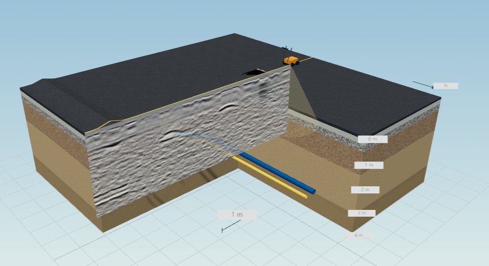
1. Know the site. Step one: know the site. Before going out, get the utility plans, which in Belgium means KLIP and KLIM-CICC, then visit the site. This is a fictitious street. Under the road there are base layers and soil, with a water main, a gas main, a utility trench, a chamber and tree roots. Making the layers transparent shows where these run. On a real site you cannot see this; that is the question the radar has to answer.
2. Choose the antenna. Step two: choose the antenna. Frequency is the key trade-off: the higher the frequency, the finer the detail, but the shallower the reach. 900 megahertz suits shallow detail. 200 megahertz reaches deeper, but small targets become hard to separate. Utility work commonly uses 400 megahertz, so we choose that here.
3. Plan the lines. Step three: plan the lines. Radar sees best what it crosses, so lines should run as square as possible to the pipes you are looking for. We start with one line, 12 metres long. The arrow on this plan shows the line and the walking direction.
4. Acquire. Step four: acquire. The radar moves along the line while the antenna sends short electromagnetic pulses into the ground. The wave reflects wherever the material changes, and the radar records when each echo returns and how strong it is. Every short step gives one trace. Trace by trace, they build up the radargram, also called a B-scan.
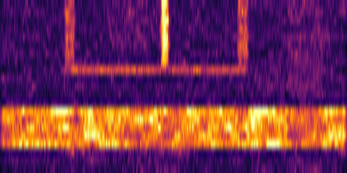
5. Read the radargram. Step five: read the radargram. Across is distance along the line. Down is two-way travel time: the later the echo, the deeper the reflector. Look at this hyperbola. As the antenna approaches a pipe the distance shrinks, then it grows again, which draws an arch. The top of the arch is directly above the pipe. So reading a radargram starts with finding these hyperbolas. Flat reflections are usually layer boundaries. Below is one single trace, the A-scan, and its spectrum. A radargram is hundreds of these side by side.
6. Process. Step six: process. In the raw record, the strong direct wave from the ground and antenna hides much of the detail. Removing the background, the part common to all traces, makes the hyperbolas stand out. Waves weaken with depth, so gain brings up the deep signals. Too much gain amplifies the noise as well.
7. Velocity and depth. Step seven: velocity and depth. Radar measures time, not depth. To convert, you need to know how fast the wave travels in this ground. Click the top of a hyperbola, then adjust the velocity until the theoretical curve fits the real one. That velocity is the wave speed in this soil. Depth equals velocity times time, divided by two.
8. Grids and time slices. Step eight: grids and time slices. One line gives one section, and it cannot show which way a pipe runs. So we survey many parallel lines over the same area, here sixteen lines, half a metre apart. Combining the energy at the same time on every line gives a plan view called a time slice, like looking down at one depth. Between about 0.5 and 0.8 metres, this wide band is the utility trench. Further down, at about one metre, the water main appears, including its bend, which a single section would never show.
9. Interpret. Step nine: interpret. List each target with its position, depth and how confident we are. The simulator knows the true answer, so we can check: the water main and the trench are clear, and the tree roots are just detectable. The polyethylene gas main and the small plastic connection were not seen: their contrast with the soil is too weak. That is a real limit of radar, and clients must be told.
10. Deliver. Step ten, the last one: deliver. On a real survey, findings are marked on the ground with spray or pegs, and the client receives radargrams with depths and confidence grades, a plan in Belgian Lambert 2008, and a report. This is the report the simulator produces: objects, verdicts and reasons together, ready to print as a PDF. Remember two things. Radar complements KLIP and KLIM-CICC plans; it does not replace them. And radar cannot tell whether a cable is live.
What it is for
One model of the site, four questions it answers.
Is radar the right tool here?
Which frequency, how deep it will reach in this soil, and which targets are likely to be missed. We use it ourselves before we quote a survey.
Compare instruments on the same line
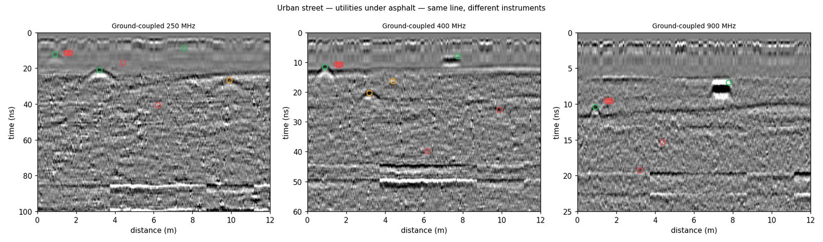
Run several radar profiles over the same site and put the radargrams side by side: depth against detail, in the ground you actually have.
Data with the answer attached
Every target comes with its true position and depth, so processing chains and automatic detectors can be checked against the truth. Labels for detector training are exported too.
Learn to read a radargram
In exercise mode the answers are hidden: students mark the reflections, fit a hyperbola for the velocity, then check their depths against the model.
From a site description to a report
Everything runs in the browser; nothing to install.
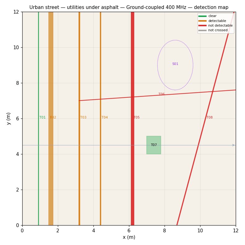
Start from an example, a form or your utility plan
Example sites — street, road, garden with old foundations, archaeological field, concrete slab, bridge deck — or a short form: surface, soil, water table and the pipes and cables you expect. A KLIP plan or a DXF drawing can be imported as the starting point.
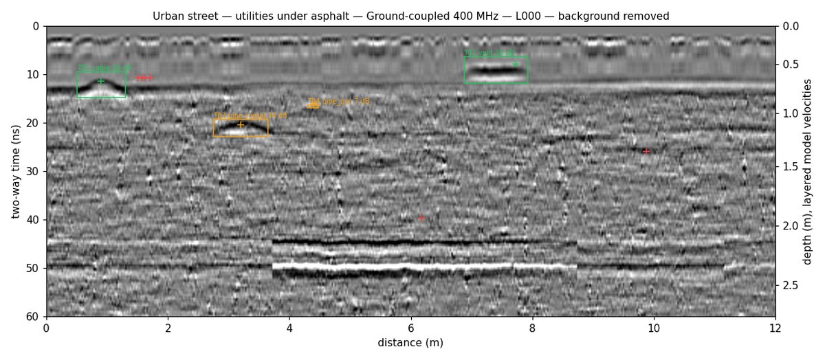
Lines and grids, as you would walk them
Single lines, parallel grids and cross grids, with the radar settings you would use on site. The result is a radargram per line, with the true targets drawn on it when you want to see them.
Every object, with a plain verdict
For each object: clear, detectable, uncertain or not found, with the reason in words — too deep for this radar in this soil, a small plastic pipe, a cable running along the line, hidden by stones and roots, or simply not crossed. Grids also give time slices.
Files your software already opens
A printable report, a findings table, radargrams as SEG-Y and DZT files (they open in RsGprProc), time slices with world files for GIS, and a DXF of what was found.
A model estimate, not a measurement
The simulator follows the physics that decides what radar sees: how fast the wave travels in each layer, how much it loses in wet or clayey ground, how strongly each object reflects, and how stones, roots and the antenna itself add clutter. Three of the radar profiles are tuned against our own field recordings, and each profile shows whether it is field-calibrated, extrapolated or based on typical values.
It does not replace a survey. Moisture changes from week to week, sites hold objects nobody drew, and live cables are best confirmed with a cable locator. Like a GPR survey, it complements the KLIP (Flanders) and KLIM-CICC (Brussels and Wallonia) plans — it does not replace them.
Access
For your organisation
quoted per organisationAccounts by invitation, a daily simulation allowance agreed with you, results kept for a period set per organisation and then deleted.
Before a survey with us
on requestWhen a site is doubtful, we can simulate it before quoting and tell you what radar is likely to find there — and what it is likely to miss.
Teaching
quotedAccounts for a class, with exercise mode for reading radargrams.
Frequently asked
Are the radargrams real measurements?
No. They are computed from a model of the site, and every simulated figure says so. They show what a given radar is likely to record; the survey on site gives the real answer.
Which radars can I simulate?
Nine profiles: ground-coupled antennas at 200, 250, 400 and 900 MHz, our own 400 MHz and 900 MHz radars, a 2 GHz concrete scanner, a 1 GHz air-launched horn and a 16-channel 600 MHz array. Antenna settings such as time window, samples and trace spacing can be changed.
Can I start from my own site?
Yes: describe it in the short form, import a KLIP plan or a DXF drawing, or have us build the site with you.
Can I open the results in my own software?
Radargrams are exported as SEG-Y and DZT files, which most processing software reads, including RsGprProc. Time slices come with world files for GIS, and findings as a table.
Check a site before you send a crew
Tell us about the site and the radar you have in mind; we will set up access or run the simulation with you.